
More Information
Submitted: January 27, 2023 | Approved: February 06, 2023 | Published: February 07, 2023
How to cite this article: Pereira J, Raposo H, Farinha JT, de-Almeida-e-Pais JE. Physical assets life cycle analysis in a food industry company - case study. Arch Food Nutr Sci. 2023; 7: 012-029.
DOI: 10.29328/journal.afns.1001045
Copyright License: © 2023 Pereira J, et al. This is an open access article distributed under the Creative Commons Attribution License, which permits unrestricted use, distribution, and reproduction in any medium, provided the original work is properly cited.
Keywords: ISO 5500X; Life Cycle Costing (LCC); Energy efficiency; Asset replacement; Asset management; Physical assets; Sustainability; Circular economy

Physical assets life cycle analysis in a food industry company - case study
João Pereira1, Hugo Raposo1-3* , José Torres Farinha1,2 and J Edmundo de-Almeida-e-Pais3,4
1Higher Institute of Engineering of Coimbra, Polytechnic of Coimbra 3030-199 Coimbra, Portugal
2Centre for Mechanical Engineering, Materials and Processes (CEMMPRE), University of Coimbra, 3030-788 Coimbra, RCM2+ - Higher Institute of Engineering of Coimbra, Polytechnic of Coimbra, Polytechnic of Coimbra, 3030-199 Coimbra, Portugal
3EIGeS - Research Centre in Industrial Engineering, Management and Sustainability. Lusófona University, Campo Grande, 376, 1749-024 Lisboa-Portugal
4CISE - Electromechatronic Systems Research Centre, University of Beira Interior, Covilhã, Portugal
*Address for Correspondence: Hugo Raposo, Instituto Superior de Engenharia de Coimbra, Polytechnic of Coimbra, 3030-199 Coimbra, Portugal, Email: [email protected]
Monitoring the life cycle of physical assets (PA) implies addressing issues, such as PA’s energy efficiency and its replacement and definition of the most proper moment to renew. The goals of this article are: to present a characterization of energy sources and analyze the PA life cycle in a food sector company. First, it will be characterized the costs and the expenses of the organization’s energy sources, then, a study about the replacement of PA is presented; Traditional methods were used, such as economic life; The models that underlie it are discussed throughout the article, using actual data, for validation. Three methods for depreciation of PA are used: Linear Depreciation; Sum of Digits and Exponential. Other methods were used to determine the Economic Cycle for replacing PA: Uniform Annual Expenditure (MRAU); Minimizing the Average Total Cost (MCMT); and the MCMT-Reduced to Present Value (MCMT-RVP). The equipment of the study was bakery ovens (gas and electrical). Results and conclusions from the application of the methods used in the evaluation of these PAs are presented.
Highlights
- Econometric models applied to physical assets’ Life Cycle to define the best time for a replacement.
- Analysis of the LCC of equipment of food industry - Case study.
- Models to increase availability and efficiency and contribute to increasing productivity.
- Monitoring/data collection of equipment to Increase productivity/quality of products.
The organization´s strategic physical asset management must reflect the organization’s objectives that underlie technical and financial decisions, including the respective plans and tactical measures, reflected in its activity plans [1].
Many organizations take decisions, not well supported, reacting to events, which means that each decision is made and implemented, sometimes by empiricism, without an analysis made about the impact that each decision will have on the organization.
In the past year energy acquired great importance in sustainability development [2] and a concern is how to move from sustainability to sustainable development [3], on our day’s development is translated on the technological increase [4], it is important to rationalize the use of energy in order to sustainable development.
Nowadays authors emphasize the need for accurate information and instruments to obtain information from assets [5,6], some bring the need to use multivariate analyses to reduce and bypass errors [7], while others rely on Artificial Intelligence (AI), to obtain solid data [8,9].
When considering energy efficiency is important to be aware of changes in the physical assets [10], does changes can be related to technological backwardness or poor maintenance.
Simple issues, such as cost, risk, and performance, are not taken into account, which can turn into a decision that seems simple to solve a given problem but corresponds to a bad decision for the organization as a whole.
Energy management – energy efficiency
Today, the concepts of Energy and Energy Efficiency are very important, both for industry and for other sectors.
Energy, according to ISO 50001:2018, is “Electricity, fuels, steam, heat, compressed air, and other forms/vectors”. The concept of energy, according to the same source, can be applied to all forms of energy including renewable ones, that is, they can be acquired, stored, processed and used in an equipment/process or even recovered.
According to Directive 2012/27/EU, Energy corresponds to “All forms of energy products, i.e., fuels, heat, renewable energy, electricity, or any other kind of energy”, as defined in the 2nd article, paragraph d), of Regulation (EC) Nº. 1099/2008 of the European Parliament and the Council of 22 October 2008 on energy statistics.
In ISO 50001:2018, it is possible to define energy efficiency as “optimizing the quantitative relationship between performance, service, good or energy and energy consumption, that is, it provides quick benefits for an organization, maximizing the use of energy sources and assets related to energy, thus reducing energy cost and consumption to provide the same amount of energy value”. The same source states that both the consumption and the results need to be specified in quantity and quality and must be measurable. Some examples are, energy efficiency/energy used; the relationship between the result/and energy consumed; among others [11].
Different authors have shown concern about energy efficiency in their research [12,13] and compare the use of classic technology to the latest one, comparing costs and environmental conditions.
According to International Energy Agency (2020), the Efficient World Strategy suggests that to unlock the full potential of efficiency, global investments would need to double by 2025, and double again by 2050. Although there are some advances in several areas, in 2018, investments are far from the results of the Efficient World Strategy. “Energy efficient financing trends can be examined by taking stock of how much was invested in efficiency in 2018 and how policies and standards enabled these investments in four key areas [14]:
- Incremental spending on more efficient technologies;
- Project investments by energy service companies (ESCOs);
- Green mortgages, green bonds, and property-based repayment schemes;
- Climate mitigation investments by international financial institutions (IFIs)”.
Recent evidence points to the role that energy efficiency has been playing, and still plays, being a central role in the world economy. In the industry, there is a high complexity regarding energy efficiency, facing great difficulties in implementing energy management.
Energy management applies to resources, such as the supply, conversion, and use of energy. It involves monitoring, measuring, recording, analyzing, controlling, and directing the flows of matter and energy to systems; so, this better energy management can be spent to achieve appreciable goals. This can be defined as the systematic activities, procedures, and routines of an industrial company, including the elements of strategy/planning, implementation/operation, control, organization, and culture, involving all support processes, with the objective of continuously reducing the consumption of the company’s energy and the related energy costs.
Energy management in companies has the following general objectives:
- Control energy consumption;
- Reduce energy costs;
- Improve working and production conditions;
- Meet government guidelines;
- Reduce CO2 emissions.
The main steps in energy management analysis are as follows:
- Energy audit
An energy audit is defined as collecting and analyzing (critical and detailed) the conditions of the power utilization of a particular equipment, process, or facility and identifying where, when, and how the energy resources are used. It also makes it possible to locate sources of energy waste, as well as to classify the efficiency of the equipment present in each facility, with the aim of determining viable technical and economic solutions and measures for the detected anomalies that allow improving the efficiency in the use of energy.
The goals of an energy audit are: to characterize the type of energy resources used; to evaluate and quantify energy consumption by sector, process, equipment, and even, facilities; to evaluate energy generation, transformation and utilization systems; relate energy consumption to production and emissions, as well as optimizing the replacement of process equipment with more efficient ones, or change the energy source (if appropriate) and thus define management strategies in order to find energy saving opportunities.
The results of the energy audit depend on the type of facilities and the objectives carried out; that is, if an audit is carried out on an office building, more importance will be given to lighting needs or ventilation systems. As in the industrial sector, the requirements of the process will be emphasized. It is important to consider the field of action and the dimensions of the audited area. To meet all the objectives of an energy audit, it should be taken into consideration the following stages: preparation of the intervention; on-site intervention; the processing of the data.
- The decision to invest in energy efficiency measures
Investments in energy efficiency are considered part of the decision-making process of the capital budget. These investments must be considered like any other investments, which means that they must be evaluated using economic evaluation tools. However, an investment in energy efficiency differs from other investments since its revenues are generated by energy savings and not by the activities that constitute the company’s core business.
According to Aragón, et al. (2013), the Key Performance Indicators (KPI) used to evaluate energy efficiency investments are the Net Present Value (NPV), the Internal Rate of Return (RoR), and the Payback. Although there are numerous criteria, Payback, and Return on Investment (ROI) are specific KPIs that may lead to wrong decision-making, while the RoR and NPV give more effective results [15].
The same authors refer that, in more recent studies, the applied methodology is Payback; this method is simple when it is used as a decision rule to reduce risk in short recovery periods. However, its use is questioned for its disadvantages, arising from the boundaries created by limiting the analysis of short periods in the recovery of investment, due to the lack of more sophisticated and accurate evaluation methodologies [15].
- Implementation of energy efficiency measures
This step is where the energy efficiency solutions are identified, particularly in terms of the thermal behavior at the plant, the renewal and/or upgrade of technical systems installed, the renovation of lighting systems, and the implementation of renewable energy systems [15].
However, to reduce energy consumption, it is possible to implement solutions, such as follows:
- Replacement of existing lighting with a more efficient one;
- Installation of motion sensors and lighting control;
- Installation of astronomical clocks that adjust the external lighting to the time of the year;
- Replacement of the existing frames with thermal cut and ventilation grilles, with double glass and low emissivity;
- Deploy isolation on roofs and walls from the outside (for example sandwich panel; underlay, etc.);
- Replacement/Acquisition of more efficient equipment;
- Installation of condenser batteries to reduce the consumption of reactive energy;
- Replacement of individual air conditioning systems by centralized systems.
In this study, regarding energy efficiency, just one detailed analysis will be made about the main energy sources used in the organization. It is important to emphasize that electricity is the most used energy source in the company. In order to compare the consumption of electricity and propane gas, a comparative analysis of both will be made. In the next section, it is discussed the best moment for the replacement of equipment, in this case, the bakery ovens.
Asset management
The term “asset” has come to be used a lot in today’s society; however, it has several meanings, depending on the area or sector concerned. An asset is a good or an entity, tangible (in the case of physical, financial, and or human assets) or intangible (in the case of software, knowledge, rights, or brands), which brings value to an individual or organization [16].
It is possible to identify five types of assets, namely [11,12]:
- Physical assets - are the facilities, equipment, and machines, among others;
- Human assets - correspond to knowledge, skills, responsibility, and experience;
- Financial assets - correspond to the earnings, financial capital, stocks, working capital, and debt;
- Intangible assets - correspond to reputation, morals, social impact, image, external relations;
- Information assets - are the data in digital format, the corporate information of the organization and the customers, and the information on financial performance.
The set of physical assets is considered by several authors the basis for the operation of companies providing services or products, as is the case of the food industry.
The purpose of asset management is not to act on assets, but on the use of them to achieve specific objectives of a company.
Asset management is defined as the set of “systematic and coordinated activities and practices through which an organization optimally and sustainably manages its assets and asset systems, performance, risks, and associated expenses, throughout its business cycles, with the objective of achieving its strategic organizational plan”.
Finally, according to the standard (ISO 55000: 2014), asset management is the “coordinated activity of an organization to perceive and produce value from assets. In this case, the perception and production of value comprise, usually, the balance of costs, risks, performance opportunities, and benefits and activity, which may include the approach, the planning, the plans, and their implementation” [17].
Based on the definitions presented above, it is possible to state that asset management is a strategic discipline that aims to “closely” monitor the assets cycle, considering the Return on Investment (ROI) attained and the achievement of social, environmental, and/or economic objectives.
Asset management brings rigor and responsibility to organizational decision-making when confronted with the following questions [17]:
- How, where, and in what to invest?
- What are the critical assets?
- What risks need to be managed?
The relationship between an asset management system and asset management is exemplified in Figure 1, where it can be seen how and where it should be placed in an organization.
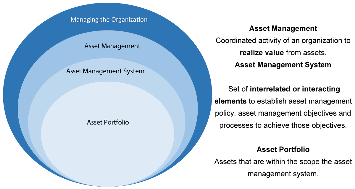
Figure 1: The relationship between management and the key concepts of asset management, (Source: ISO 55000:2014).
While not all organizations are able to implement an asset management system, time is running out, and its implementation becomes more and more critical to their survival. The application of an asset management system consists of a set of objectives that can be achieved in a consistent and sustainable way over time. For an organization to have good Asset Management, it must be present across all stakeholders. Through development of appropriate methodologies, the evolution of Asset Management must be developed over the years, thus making organizations more efficient [18].
Physical assets: Equipment replacement is among the mandatory and relevant decisions that are made throughout the organization’s life, especially in industries. The mistakes occurred after making these decisions may compromise the survival of companies. Late or premature equipment replacement leads the organization to have financial losses [19].
The first step to effectively start managing physical assets is to know the detailed data of all existing assets, their importance,s and criticality.
To address this issue, it is necessary to know a set of factors, such as [20]:
- Asset’s name and characteristics;
- Configuration (summary);
- Location;
- Age;
- Condition;
- Life Cycle Duration (estimate);
- Replacement cost;
- History;
- Known problems;
- Known plans.
The group of factors should be complemented with maps, photographs, and diagrams, among other details, to assist in the identification of the location and condition of the assets.
The collection of this data, as well as the existence of a good record of all significant events throughout the asset’s useful life, will allow that, in the future, will be a more reliable information support for the assessment of their capacity to face the requirements of the Stakeholders, as well as for the preparation of technical-economic studies of possible investments.
According to Raposo, et al. [21], the life cycle cost (LCC) of an asset is the sum of all capital spent to support that asset from the conception phase, through the operations e maintenance phase to the end of its useful life.
Econometric substitution models: Many companies keep equipment running when their operation is no longer economically viable, as they don´t know the LCC of the equipment [21]. This has numerous implications; in the case of the food industry, for example, it has direct implications for the efficiency of the equipment.
According to Raposo, et al. [22], the analysis of the life cycle of physical assets and, particularly, the support for the decisions of acquisition, replacement, or equipment obsolescence, should take into consideration the investment methods.
There are several mathematical models that allow making the appropriate characterization to determine the most rational time for the equipment replacement. For this, it is necessary to consider certain variables, such as [23]:
- Acquisition Cost (CA);
- Value of Assignment (VC);
- Operating Cost (CE);
- Maintenance costs (CM);
- Operating cost (CO).
- Inflation rate (θ);
- Capitalization Rate (i).
The values of most of the preceding variables are obtained through history, except for the assignment value. In this case, it will be necessary to obtain the market value for each specific piece of equipment, which may be difficult to reach for many assets. Regulatory decreet number 25/2009, of September 14, corresponds to the regulatory regime for depreciation and amortization that establishes the appropriate depreciation method as well as the depreciation and amortization rates for each physical asset.
As an alternative to this decree-law, various types of devaluation can be simulated, such as [1,13,14,18]:
- Linear Depreciation Method - the devaluation of the equipment value is constant over the years;
- Sum of Digits Method – the annual depreciation is non-linear;
- Exponential method - the annual depreciation value is decreasing over the equipment’s life.
Asset replacement methods: According to Raposo, et al. [3], the equipment can be replaced for several reasons. On the financial side, a common criterion is the “economic cycle”, which allows for determining the optimum period that minimizes the total costs of operation, maintenance, and capital immobilization.
Another method, widely used, is that of “useful life”, which defines that it ends when its maintenance costs exceed the maintenance costs plus the amortization of the capital of equivalent new equipment.
However, if possible, this doesn’t prevent making an equipment replacement analysis from market depreciation, which should consider two other types of variables [23]:
- The capitalization rate, denominated by i;
- The inflation rate, denominated by θ.
These rates are related as follows:
iA = i + θ + i * θ (1)
Being,
iA - Apparent rate
There are several methods for determining the economic cycle for equipment replacement. The most used are the following [17]:
- Uniform Annual Expenditure Method (MRAU);
- Average Total Cost Minimization Method (MCMT);
- MCMT method with reduced present value (MCMT - RVP).
Case study – food industry
In the first part, the analysis of the energy consumption of both energy sources in the organization is presented. As previously mentioned, the energy sources covered are electric energy and propane gas. In this way, an analysis/evaluation was made about the consumption and costs of the company’s energy sources; in the second part, several models are presented that allow supporting the decision about the best time to replace an asset. In this phase, a survey of the historical data relating to two ovens (Ring Oven and Electric Oven) was carried out. Based on this database, the study of an integrated replacement model for the company’s ovens is done.
Energy management – Energy Efficiency
In this section, a comparative analysis of the company’s energy sources is made. Currently, companies are looking for energy efficiency with the aim of reducing invoice value and being less polluting. For this, it was necessary to carry out a small survey to characterize each oven used in the study.
View of the cost of the organization’s energy sources over the years: As can be seen in Figures 2,3, the price of electricity and propane gas is inconsistent.
About Figure 2, as observed the price per kWh tends to increase consistently, but the same cannot be said about Figure 3, where it can be seen some fluctuation in the price of propane gas over the years.
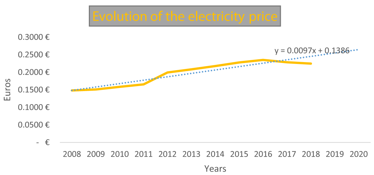
Figure 2: Evolution of the electricity price.
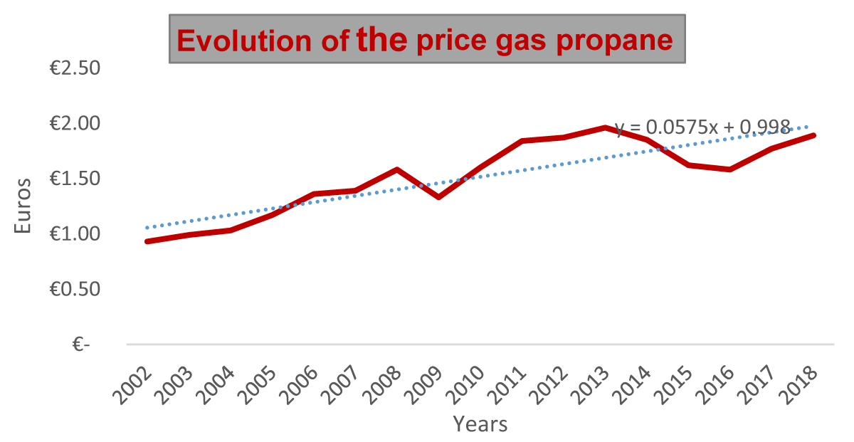
Figure 3: Evolution of the price of gas propane.
View of the cost analysis of the invoiced cost of energy sources: In Figures 4,5 can be observed the costs of electricity and gas sources, respectively, in the last five years.
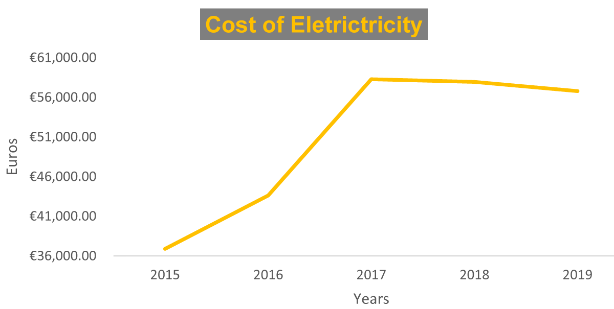
Figure 4: Electricity charges over the years.
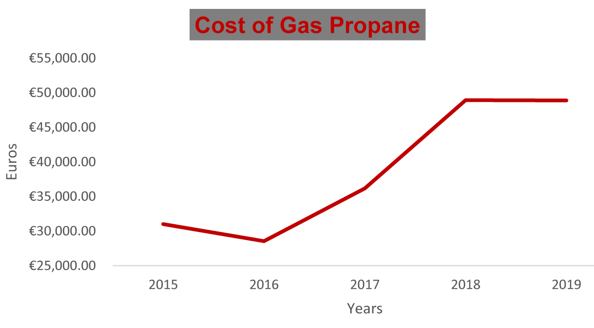
Figure 5: Gas propane charges over the years.
In Figure 4, as can be seen, from 2016 to 2017, there was a significant increase in electricity costs. This is due to the increase in the number of refrigerated rooms and storage rooms for frozen and refrigerated products. After noticing the annual energy costs in 2017, they implemented some measures, which have been pointed out in 2018 and, subsequently, in 2019. In Figure 5, it is observed that the cost of gas suffers some oscillations over the years. The oscillations verified are directly related to the annual variation in the price of gas, that is, these oscillations do not depend on the increase in production.
As expected, energy consumption is not constant over the years, that is, it depends on factors, such as weather conditions, because in the hotter years, the refrigeration/freezing equipment makes a greater effort to maintain the appropriate temperature in the cold rooms, the variability of the production load, due to the peak production at Easter and Christmas, among others.
In order to understand the energy needs of the organization, it is important to survey the history of energy consumption. As previously mentioned, the data used were from the last five years, that is, from 2015 to the present date. Although the amounts paid are monthly, it does not mean that the billing period is from the 1st to the 30th of each month. Based on the preceding and the analysis of Table 1, it is possible to observe the company’s annual energy consumption and the amounts paid to energy suppliers.
Based on the analysis of Table 1 and Figure 6, it is possible to verify what had previously been found, namely because in 2016 and 2017 there was a significant increase in power consumption.
| Table 1: Participants characteristics and P wave dispersion, Left atrium and Ejection fraction values | ||||
| Table 1: Electricity consumption converted into TEP. | ||||
| year | Active energy consumed (kWh) | total cost (€) (with IVA) |
average cost (€/kWh) (with IVA) | Conversion to tep |
| 2015 | 375 762,97 | 36 887,27 | 0,098 | 80,8 |
| 2016 | 435 352,61 | 43 617,66 | 0,100 | 93,6 |
| 2017 | 552 709,07 | 58 277,58 | 0,105 | 118,8 |
| 2018 | 570 473,44 | 57 945,73 | 0,102 | 122,7 |
| 2019 | 551 261,35 | 56 777,43 | 0,103 | 118,5 |
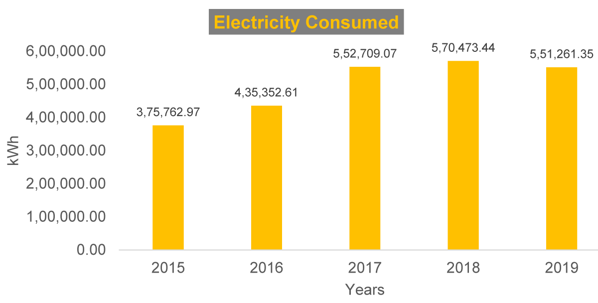
Figure 6: Electricity consumed annually.
This increase was due to the expansion of the facilities, where more air-conditioned areas were created. It is also noted that some of the measures implemented were effective in reducing energy consumption, as there was a decrease in this consumption from 2018 to 2019.
It is also verified that there is great variability in energy consumption throughout the year (Figure 7), being possible to verify that, in the summer months, there is an increase in consumption, which is due to the average ambient temperature in those months being higher than the rest of the year. It is important to note that the company’s administration monitors the energy costs, which is reflected in changing the energy provider over the years.
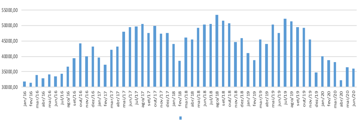
Figure 7: Monthly electricity consumption over the 5 years.
The data on gas consumption was more difficult to obtain, since, unlike electricity consumption, where there is a management platform, here we can only calculate the consumption of propane gas through the amount paid to the gas operator and the average cost per kilogram of gas. Thus, through the analysis of Table 2 and Figure 8, it is possible to verify that there were also significant increases in gas consumption in the years 2017 and 2018. These increases are a consequence of the increase in production and greater use of gas ovens.
| Table 2: Gas propane consumption converted into TEP. | ||||
| Year | Gas propane consumed (kg) | Total cost (€) (with IVA) | Average cost (€/kg) (with IVA) | Conversion to TEP |
| 2015 | 137 813,11 | 31 007,95 | 0,2250 | 153,6 |
| 2016 | 122 364,32 | 28 535,36 | 0,2332 | 136,4 |
| 2017 | 149 781,61 | 36 172,26 | 0,2415 | 166,9 |
| 2018 | 195 915,86 | 48 920,19 | 0,2497 | 218,3 |
| 2019 | 184 472,25 | 48 883,84 | 0,2580 | 210,1 |
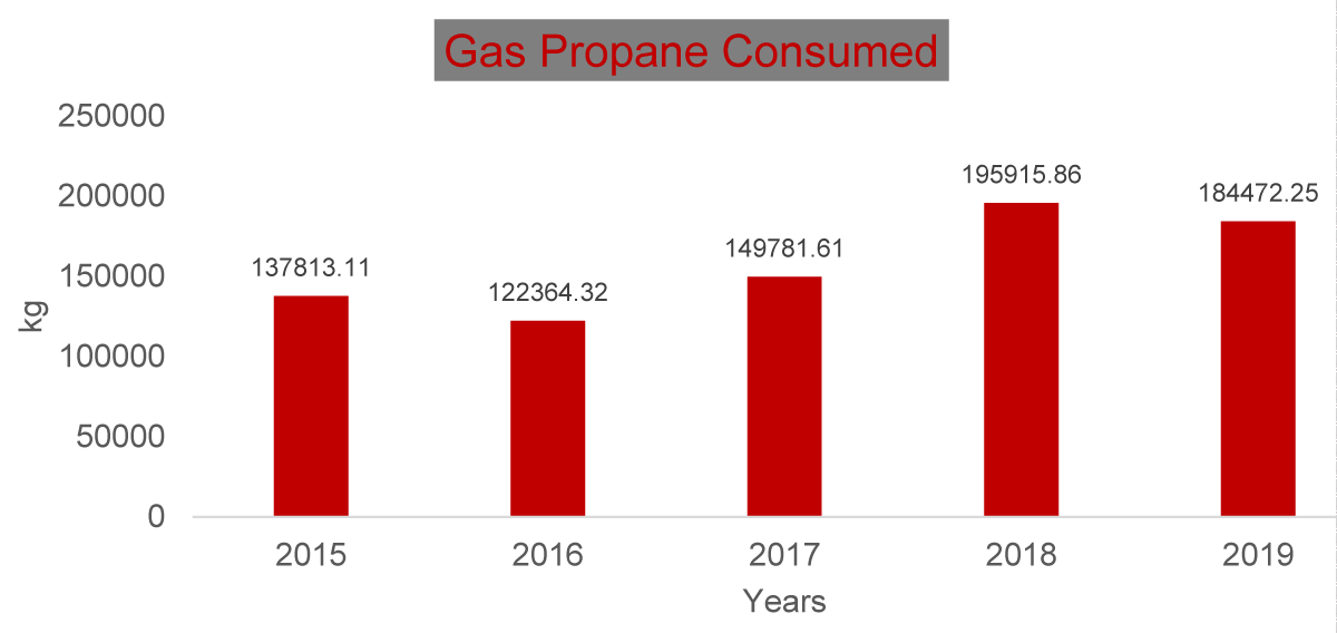
Figure 8: Gas propane consumed annually.
In order to check if the company is covered by the SGCIE, the consumption of energy sources has been converted to TEP, from the last five years.
From the analysis of Table 3, we can see that the company is not covered by the SGCIE since the active energy consumption does not exceed 500 tep. Therefore, we can say that the company is not considered an intensive consumer of energy.
| Table 3: Total energy consumption into TEP. | ||
| Consumption of the energy sources | ||
| Electricity (tep) | Gas propane (tep) | Total (tep) |
| 80,8 | 153,6 | 234,4 |
| 93,6 | 136,4 | 230 |
| 118,8 | 166,9 | 285,7 |
| 122,7 | 218,3 | 341 |
| 118,5 | 210,1 | 328,6 |
Measures implemented for energy efficiency: At the beginning of the study for the project elaboration, the organi-zation had already implemented some measures, namely:
- Replacement of halogen lighting with LED lighting;
- Installation of motion sensors and lighting control;
- Installation of astronomical clocks in order to turn on or off according to their use, in ovens, greenhouses, and outdoor lighting;
- Placing insulation on the covers and walls (sandwich panel);
- Installation of capacitor battery to reduce reactive energy consumption.
During the elaboration of the project, some of the measures taken were:
- Replacement of Chambers - Bearing in mind that the objective of increasing the number of areas was not fully completed, that is, it did not increase production, nor was possible to produce other products for another type of market, then, it was decided to replace the old chambers by others of more recent technology. This replacement consists of turning off the old chambers and turning on the new ones, which are characterized by being more energy efficient and being directed to a centralized system;
- Switching off Electric Oven # 1 - This oven is used during the night shift, and, after use, it is switched off. After a few days of observation, it was found that bakers turned on the electric oven nº1 around 10 am, to cook certain products that could be cooked in the ring oven. Having said that, and taking into consideration the fares and schedules cycles, bakery and pastry furnace operators were warned that the electric oven was not to turn on after 8 am, since, from that time, it entered working full time. This type of equipment, at the time of start-up, uses a high amount of energy, which caused the daily consumption of energy (kWh) to skyrocket. After taking this measure, we observed one significant reduction in energy consumption (MWh), as illustrated in Figure 9; based on this, it is possible to see a monthly decrease in energy consumption (MWh), compared to 2018. According to the presented data, in May and November, there is an increase of about 2% in relation to 2018, a fact which can be explained by the slight increase in production. In relation to the month of July of the year 2019, there is an increase of 4% in energy consumption due to a malfunction in the ring furnace.
- Turn off some equipment after use - Employees had an old habit of turning on the equipment at the beginning of the shift and off only at the end of each shift. After checking for some occurrences (which could be avoided), the rule was implemented that, when someone finished a task with a certain piece of equipment, they should immediately turn it off. The equipment covered by this rule is equipment that does not require a large amount of energy to start a specific task. Examples of this are mixers, kneaders and laminators.
Asset management – asset replacement
This subsection presents a case study to determine the most appropriate time to replace an oven, using replacement econometric models, considering the influence of endogenous and exogenous variables. For a better understanding of the analysis carried out, some examples of the determination of that moment are presented, referring to the auxiliary calculations of the models presented.
At this phase, managers, engineers, and general employees must actively engage in the analysis and collection of data, as no one is better than these to know which criteria are considered important for the company’s strategic and economic planning and which directly affect the performance of the equipment. Some examples of criteria are operation, maintenance, etc.
First, the data collected will be analyzed at an apparent constant rate and then at an apparent variable rate over the years. This analysis will determine whether the apparent rate influences the final results.
Electric oven
- Oven characterization
On its nameplate, can be checked the entire identity of the electric oven (Figure 10). As can be observed, the oven was installed in 2008 and is a device, approximately, 13 years. The nameplate indicates a power of 49kW, information that will be used for the calculation of costs. As seen in Figure 11, marked in white, it is an equivalent oven; however, this one is more economical than expected.
The data in Table 4 was collected for the electric furnace and is used for calculating methods of asset replacement.
| Table 4: Equipment History (electric oven). | |
|
16.200,00€ |
|
2008 |
|
Ramalhos |
|
25 years |
|
1.000,00€ |
- Calculation of Maintenance and Operation Costs
Due to the uncertainty of data collected concerning the maintenance costs (Table 5), it was decided to:
| Table 5: Maintenance costs of the electric furnace. | ||
| Electric Oven- 3C/2P | ||
| Year | Type of Service | Cost |
| 2011 | Factory Utensil Tools | 359,18 € |
| 2013 | Factory Utensil Tools | 215,80 € |
| Equipment Maintenance Repairs | 37,35 € | |
| Freight Transport | 9,89 € | |
| 2014 | Tempered Glass | 43,59 € |
| Freight Transport | 9,89 € | |
| 2016 | Equipment Maintenance Repairs | 57,81 € |
- Considering that we have no real data on the maintenance costs – it is assumed that, in the first year (2009), the cost of maintenance is 1.000,00 € and, as of 2010, an increase of 10% was considered in relation to the average cost (under the history of data collected);
- Assume the average monthly cost of electrical work (including hours of maintenance electrician + equipment) of 50,00 € (Table 6).
| Table 6: Average Maintenance Cost. | |
| Maintenance Cost | |
| Maintenance Cost - Electrician | 600€ |
| Average Cost (over the years - historical) | 104,79 € |
| Total | 704,79 € |
Regarding the operating costs of the electric furnace, they only considered the energy costs; thus, it was necessary to collect data on the variation of electricity prices over the years. Database in Portugal that provides this type of information, it is considered that both worked 11 hours daily and only 361 days a year, as the company closes on 25 and 26 December, and on 1 and 2 January also (Table 7).
| Table 7: Operation cost. | |
| Operation Cost | |
| Number of hours (work) | 11h |
| Overpower | 49 kW/h |
| Number of working dayS | 361 days |
Based on Table 8, we can predict the estimated values of the cost of energy for the coming years, as well as the total costs of maintenance and operation.
| Table 8: Operation and maintenance cost of the Electric Oven. | ||||||
| Year | Cost (€ /kw) |
Cost | Operation Cost |
Maintenance Cost |
Total | |
| 2008 | 0 | 1,6302 € | 6 473,52 € | 7 473,52 € | ||
| 2009 | 1 | 0,1508 € | 1,6588 € | 6 587,09 € | 1 000,00 € | 7 473,52 € |
| 2010 | 2 | 0,1584 € | 1,7424 € | 6 919,07 € | 900,00 € | 7 487,09 € |
| 2011 | 3 | 0,1654 € | 1,8194 € | 7 224,84 € | 731,79 € | 7 650,86 € |
| 2012 | 4 | 0,1993 € | 2,1923 € | 8 705,62 € | 753,74 € | 7 978,58 € |
| 2013 | 5 | 0,2081 € | 2,2891 € | 9 090,02 € | 776,36 € | 9 481,98 € |
| 2014 | 6 | 0,2175 € | 2,3925 € | 9 500,62 € | 799,65 € | 9 889,66 € |
| 2015 | 7 | 0,2279 € | 2,5069 € | 9 954,90 € | 823,64 € | 10 324,25 € |
| 2016 | 8 | 0,2350 € | 2,5850 € | 10 265,04 € | 848,35 € | 10 803,25 € |
| 2017 | 9 | 0,2284 € | 2,5124 € | 9 976,74 € | 873,80 € | 11 138,83 € |
| 2018 | 10 | 0,2246 € | 2,4706 € | 9 810,75 € | 900,01 € | 10 876,75 € |
| 2019 | 11 | 0,2453 € | 2,6983 € | 10 714,95 € | 927,01 € | 10 737,76 € |
| 2020 | 12 | 0,2550 € | 2,8050 € | 11 138,66 € | 954,82 € | 11 669,77 € |
| 2021 | 13 | 0,2647 € | 2,9117 € | 11 562,36 € | 983,46 € | 12 122,12 € |
| 2022 | 14 | 0,2744 € | 3,0184 € | 11 986,07 € | 1 012,97 € | 12 575,33 € |
| 2023 | 15 | 0,2841 € | 3,1251 € | 12 409,77 € | 1 043,36 € | 13 029,42 € |
| 2024 | 16 | 0,2938 € | 3,2318 € | 12 833,48 € | 1 074,66 € | 13 484,43 € |
| 2025 | 17 | 0,3035 € | 3,3385 € | 13 257,18 € | 1 106,90 € | 13 940,38 € |
| 2026 | 18 | 0,3132 € | 3,4452 € | 13 680,89 € | 1 140,10 € | 14 397,29 € |
| 2027 | 19 | 0,3229 € | 3,5519 € | 14 104,59 € | 1 174,31 € | 14 855,20 € |
| 2028 | 20 | 0,3326 € | 3,6586 € | 14 528,30 € | 1 209,54 € | 15 314,13 € |
| 2029 | 21 | 0,3423 € | 3,7653 € | 14 952,01 € | 1 245,82 € | 15 774,12 € |
| 2030 | 22 | 0,3520 € | 3,8720 € | 15 375,71 € | 1 283,20 € | 16 235,20 € |
| 2031 | 23 | 0,3617 € | 3,9787 € | 15 799,42 € | 1 321,69 € | 16 697,41 € |
| 2032 | 24 | 0,3714 € | 4,0854 € | 16 223,12 € | 1 361,34 € | 17 160,76 € |
| 2033 | 25 | 0,3811 € | 4,1921 € | 16 646,83 € | 1 402,19 € | 17 625,31 € |
Table 9 and Figure 12 present the values referring to the three methods used for the depreciation of an electric oven, that are: The Linear Depreciation Method; the Sum of Digits Method; and the Exponential Method.
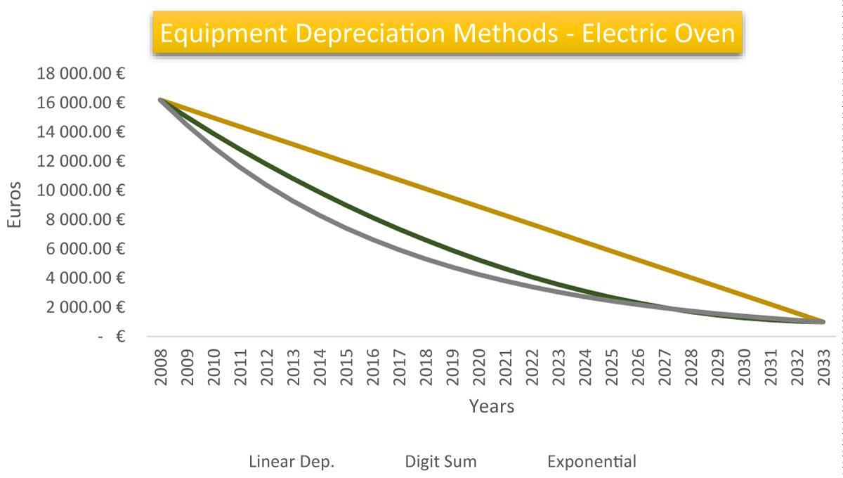
Figure 12: Equipment depreciation methods – electric furnaces.
| Table 9: Equipment depreciation methods – electric furnace. | ||||
| Year | Methods | |||
| j | Linear Dep | Digit Sum | Exponential | |
| 2008 | 0 | 16 200,00 € | 16 200,00 € | 16 200,00 € |
| 2009 | 1 | 15 592,00 € | 15 030,77 € | 14 492,20 € |
| 2010 | 2 | 14 984,00 € | 13 908,31 € | 12 964,44 € |
| 2011 | 3 | 14 376,00 € | 12 832,62 € | 11 597,74 € |
| 2012 | 4 | 13 768,00 € | 11 803,69 € | 10 375,11 € |
| 2013 | 5 | 13 160,00 € | 10 821,54 € | 9 281,37 € |
| 2014 | 6 | 12 552,00 € | 9 886,15 € | 8 302,93 € |
| 2015 | 7 | 11 944,00 € | 8 997,54 € | 7 427,64 € |
| 2016 | 8 | 11 336,00 € | 8 155,69 € | 6 644,62 € |
| 2017 | 9 | 10 728,00 € | 7 360,62 € | 5 944,15 € |
| 2018 | 10 | 10 120,00 € | 6 612,31 € | 5 317,52 € |
| 2019 | 11 | 9 512,00 € | 5 910,77 € | 4 756,95 € |
| 2020 | 12 | 8 904,00 € | 5 256,00 € | 4 255,47 € |
| 2021 | 13 | 8 296,00 € | 4 648,00 € | 3 806,86 € |
| 2022 | 14 | 7 688,00 € | 4 086,77 € | 3 405,54 € |
| 2023 | 15 | 7 080,00 € | 3 572,31 € | 3 046,53 € |
| 2024 | 16 | 6 472,00 € | 3 104,62 € | 2 725,37 € |
| 2025 | 17 | 5 864,00 € | 2 683,69 € | 2 438,06 € |
| 2026 | 18 | 5 256,00 € | 2 309,54 € | 2 181,04 € |
| 2027 | 19 | 4 648,00 € | 1 982,15 € | 1 951,12 € |
| 2028 | 20 | 4 040,00 € | 1 701,54 € | 1 745,43 € |
| 2029 | 21 | 3 432,00 € | 1 467,69 € | 1 561,43 € |
| 2030 | 22 | 2 824,00 € | 1 280,62 € | 1 396,82 € |
| 2031 | 23 | 2 216,00 € | 1 140,31 € | 1 249,57 € |
| 2032 | 24 | 1 608,00 € | 1 046,77 € | 1 117,84 € |
| 2033 | 25 | 1 000,00 € | 1 000,00 € | 1 000,00 € |
The study period for the electric oven equipment was 25 years, as, according to our experience, it is the maximum useful life of the equipment. Therefore, the study goes from the moment of acquisition until the end of the equipment’s life, that is, from 2008 (the year of acquisition) until 2033.
The annual depreciation quota of 608,00 € was obtained using the Linear Depreciation method. Under the Exponential method, the depreciation rate obtained was 10.5%.
Through the analysis of Table 9, it is possible to verify that the Linear Depreciation method has a slower decrease over time; the same does not happen with the other two methods. It is noted that, if we compare the method of the sum of the digits with the exponential method, what presents a much faster decay than the method of the sum of the digits? With the aforementioned study, it was possible to manage the data related to the economic cycle for replacing the electric oven, which data can be seen in Figure 12.
Constant apparent rate replacement methods – Electric Oven
− Uniform annual expenditure method (MRAU) – Electric Oven
The Income Annual Liquid (RAUn) is given by [21]:
(2)
(3)
Figure 13 and Table 10 show the results obtained through the application of the uniform annual expenditure method.
Figure 1: MRAU whit constant apparent rate – Electric Oven.
| Table 10: MRAU with constant apparent rate – Electric Oven. | ||||
| Year | Uniform Annual Expenditure Method | |||
| j | Linear Dep | Digit Sum | Exponential | |
| 2008 | 0 | |||
| 2009 | 1 | 8 087,60 € | 8 654,45 € | 9 198,40 € |
| 2010 | 2 | 8 097,41 € | 8 643,34 € | 9 122,36 € |
| 2011 | 3 | 8 156,77 € | 8 681,56 € | 9 101,44 € |
| 2012 | 4 | 8 268,71 € | 8 772,12 € | 9 138,24 € |
| 2013 | 5 | 8 631,83 € | 9 113,64 € | 9 430,98 € |
| 2014 | 6 | 8 941,20 € | 9 401,18 € | 9 674,37 € |
| 2015 | 7 | 9 223,29 € | 9 661,22 € | 9 894,55 € |
| 2016 | 8 | 9 493,44 € | 9 909,07 € | 10 106,56 € |
| 2017 | 9 | 9 740,05 € | 10 133,16 € | 10 298,51 € |
| 2018 | 10 | 9 912,89 € | 10 283,24 € | 10 419,94 € |
| 2019 | 11 | 10 042,85 € | 10 390,20 € | 10 501,49 € |
| 2020 | 12 | 10 225,15 € | 10 549,27 € | 10 638,16 € |
| 2021 | 13 | 10 412,62 € | 10 713,27 € | 10 782,60 € |
| 2022 | 14 | 10 604,07 € | 10 881,01 € | 10 933,39 € |
| 2023 | 15 | 10 798,59 € | 11 051,58 € | 11 089,50 € |
| 2024 | 16 | 10 995,53 € | 11 224,33 € | 11 250,09 € |
| 2025 | 17 | 11 194,38 € | 11 398,74 € | 11 414,53 € |
| 2026 | 18 | 11 394,75 € | 11 574,43 € | 11 582,27 € |
| 2027 | 19 | 11 596,33 € | 11 751,08 € | 11 752,88 € |
| 2028 | 20 | 11 798,86 € | 11 928,45 € | 11 926,02 € |
| 2029 | 21 | 12 002,16 € | 12 106,33 € | 12 101,36 € |
| 2030 | 22 | 12 206,07 € | 12 284,57 € | 12 278,66 € |
| 2031 | 23 | 12 410,44 € | 12 463,03 € | 12 457,68 € |
| 2032 | 24 | 12 615,17 € | 12 641,59 € | 12 638,24 € |
| 2033 | 25 | 12 820,17 € | 12 820,17 € | 12 820,17 € |
As can be seen that both depreciation methods follow the same trajectory and are very similar. However, it is possible to see that it is difficult, for the decision-maker, to define the exact time for the replacement of the furnace since it was not possible to obtain the time when the annual expenses were minimal. We can also mention that the use of a constant apparent rate over the years may influence the final results obtained.
− Method of minimizing average total cost (MCMT) – Electric Oven
Mathematical formula of Total Average Cost Minimization Method (MCMT) [21]:
(4)
Through the study previously carried out, this method would not bring any answer. However, through the analysis of Figure 14 and Table 11, we can verify that the method of minimizing the total average cost transmits information about the best time to replace the equipment.
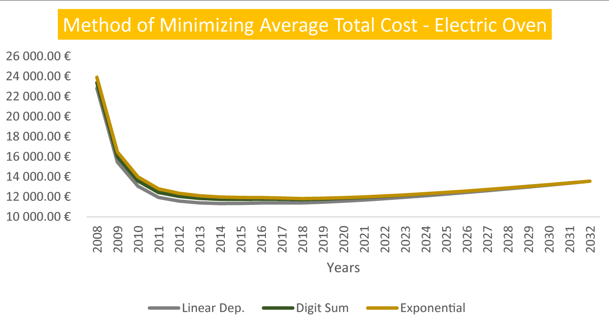
Figure 14: MCMT with constant apparent rate – Electric Oven.
| Table 11: MCMT with constant apparent rate – Electric Oven. | ||||
| Year | Method of Minimizing Average Total Cost- RVP | |||
| Civil | j | Linear Dep | Digit Sum | Exponential |
| 2008 | 0 | |||
| 2009 | 1 | 22 808,00 € | 23 369,23 € | 23 907,80 € |
| 2010 | 2 | 15 451,55 € | 15 989,39 € | 16 461,33 € |
| 2011 | 3 | 13 053,99 € | 13 568,45 € | 13 980,07 € |
| 2012 | 4 | 11 937,13 € | 12 428,21 € | 12 785,36 € |
| 2013 | 5 | 11 567,70 € | 12 035,40 € | 12 343,43 € |
| 2014 | 6 | 11 389,36 € | 11 833,67 € | 12 097,54 € |
| 2015 | 7 | 11 324,06 € | 11 744,98 € | 11 969,26 € |
| 2016 | 8 | 11 334,96 € | 11 732,50 € | 11 921,38 € |
| 2017 | 9 | 11 380,72 € | 11 754,88 € | 11 912,26 € |
| 2018 | 10 | 11 391,13 € | 11 741,89 € | 11 871,37 € |
| 2019 | 11 | 11 387,00 € | 11 714,39 € | 11 819,28 € |
| 2020 | 12 | 11 461,23 € | 11 765,23 € | 11 848,61 € |
| 2021 | 13 | 11 558,84 € | 11 839,45 € | 11 904,16 € |
| 2022 | 14 | 11 674,87 € | 11 932,10 € | 11 980,76 € |
| 2023 | 15 | 11 805,71 € | 12 039,56 € | 12 074,61 € |
| 2024 | 16 | 11 948,63 € | 12 159,09 € | 12 182,80 € |
| 2025 | 17 | 12 101,56 € | 12 288,63 € | 12 303,08 € |
| 2026 | 18 | 12 262,88 € | 12 426,57 € | 12 433,71 € |
| 2027 | 19 | 12 431,31 € | 12 571,62 € | 12 573,25 € |
| 2028 | 20 | 12 605,85 € | 12 722,78 € | 12 720,58 € |
| 2029 | 21 | 12 785,68 € | 12 879,22 € | 12 874,75 € |
| 2030 | 22 | 12 970,11 € | 13 040,26 € | 13 034,98 € |
| 2031 | 23 | 13 158,60 € | 13 205,37 € | 13 200,62 € |
| 2032 | 24 | 13 350,69 € | 13 374,08 € | 13 371,11 € |
| 2033 | 25 | 13 546,00 € | 13 546,00 € | 13 546,00 € |
By applying the linear depreciation method, the decision maker can verify that the best time to replace the electric oven is in 2015. With the application of two other two methods, it was possible to observe that the best replacement time would be in 2019. In this case, by the application of this method, the decision maker replaced the equipment in 2019.
- Method of minimizing the average total cost with reduction to present value (MCMT – RVP) – Electric Oven
Mathematical formula of minimizing the average total cost with reduction to present value (MCMT – RVP) [21]:
(5)
Through the application of this method and the analysis of Figure 15 and Table 12, it is possible to verify that there is no time when the average cost of the equipment is minimal. This means that it is not possible to identify the best time to replace the equipment using this method.
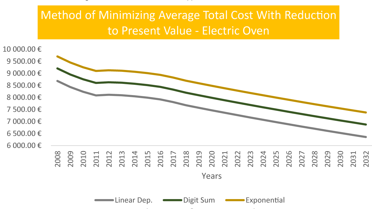
Figure 15: MCMT-RVP with constant apparent rate – Electric oven./p>
| Table 12: MCMT - RVP with constant apparent – Electric Oven. | ||||
| Year | Method of Minimizing Average Total Cost- RVP | |||
| Civil | j | Linear Dep | Digit Sum | Exponential |
| 2008 | 0 | |||
| 2009 | 1 | 8 161,91 € | 8 717,58 € | 9 250,81 € |
| 2010 | 2 | 8 131,93 € | 8 687,60 € | 9 220,83 € |
| 2011 | 3 | 8 150,69 € | 8 706,37 € | 9 239,60 € |
| 2012 | 4 | 8 220,43 € | 8 776,10 € | 9 309,34 € |
| 2013 | 5 | 8 533,17 € | 9 088,85 € | 9 622,08 € |
| 2014 | 6 | 8 790,79 € | 9 346,47 € | 9 879,70 € |
| 2015 | 7 | 9 019,54 € | 9 575,21 € | 10 108,44 € |
| 2016 | 8 | 9 234,47 € | 9 790,14 € | 10 323,38 € |
| 2017 | 9 | 9 424,75 € | 9 980,43 € | 10 513,66 € |
| 2018 | 10 | 9 543,17 € | 10 098,85 € | 10 632,08 € |
| 2019 | 11 | 9 619,88 € | 10 175,55 € | 10 708,78 € |
| 2020 | 12 | 9 744,78 € | 10 300,45 € | 10 833,69 € |
| 2021 | 13 | 9 873,15 € | 10 428,83 € | 10 962,06 € |
| 2022 | 14 | 10 003,82 € | 10 559,49 € | 11 092,72 € |
| 2023 | 15 | 10 135,91 € | 10 691,59 € | 11 224,82 € |
| 2024 | 16 | 10 268,80 € | 10 824,48 € | 11 357,71 € |
| 2025 | 17 | 10 402,01 € | 10 957,68 € | 11 490,92 € |
| 2026 | 18 | 10 535,16 € | 11 090,84 € | 11 624,07 € |
| 2027 | 19 | 10 667,98 € | 11 223,65 € | 11 756,88 € |
| 2028 | 20 | 10 800,23 € | 11 355,90 € | 11 889,13 € |
| 2029 | 21 | 10 931,74 € | 11 487,41 € | 12 020,65 € |
| 2030 | 22 | 11 062,37 € | 11 618,05 € | 12 151,28 € |
| 2031 | 23 | 11 192,02 € | 11 747,69 € | 12 280,92 € |
| 2032 | 24 | 11 320,58 € | 11 876,26 € | 12 409,49 € |
| 2033 | 25 | 11 448,00 € | 12 003,68 € | 12 536,91 € |
Variable apparent rate replacement method – Electric Oven
- Uniform annual expenditure method (MRAU) – Electric Oven
Figure 16 and Table 13 show the results obtained by applying the method of uniform annual expenditure, with the variable apparent rate. As it is possible to see through the application of these methods, there is a deviation in the values presented by them. When observing Figure 16, it can be concluded that the decision maker is able to define a time for the furnace replacement. This replacement time is in 2014, that is, it is the minimum value given by the annual expenditure method that transmits to the decision-maker the most appropriate time to replace the equipment.
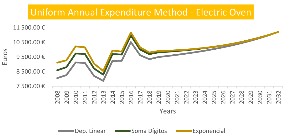
Figure 16: MRAU with variable apparent rate – Electric Oven.
| Table 13: MRAU with variable apparent rate – Electric Oven. | ||||
| Year | Uniform Annual Expenditure Method | |||
| Civil | j | Linear Dep | Digit Sum | Exponential |
| 2008 | 0 | |||
| 2009 | 1 | 8 055,02 € | 8 591,78 € | 9 106,86 € |
| 2010 | 2 | 8 260,62 € | 8 798,79 € | 9 271,01 € |
| 2011 | 3 | 9 119,55 € | 9 731,77 € | 10 221,61 € |
| 2012 | 4 | 9 095,91 € | 9 708,89 € | 10 154,70 € |
| 2013 | 5 | 8 205,76 € | 8 708,82 € | 9 040,15 € |
| 2014 | 6 | 7 865,39 € | 8 289,25 € | 8 540,97 € |
| 2015 | 7 | 9 229,04 € | 9 691,33 € | 9 937,64 € |
| 2016 | 8 | 9 235,10 € | 9 660,86 € | 9 863,16 € |
| 2017 | 9 | 10 508,22 € | 10 966,28 € | 11 158,96 € |
| 2018 | 10 | 9 616,15 € | 10 004,40 € | 10 147,72 € |
| 2019 | 11 | 9 344,34 € | 9 690,68 € | 9 801,64 € |
| 2020 | 12 | 9 492,77 € | 9 812,19 € | 9 899,79 € |
| 2021 | 13 | 9 565,43 € | 9 855,15 € | 9 921,95 € |
| 2022 | 14 | 9 643,90 € | 9 904,36 € | 9 953,64 € |
| 2023 | 15 | 9 728,90 € | 9 960,76 € | 9 995,51 € |
| 2024 | 16 | 9 821,40 € | 10 025,45 € | 10 048,43 € |
| 2025 | 17 | 9 922,53 € | 10 099,69 € | 10 113,37 € |
| 2026 | 18 | 10 033,50 € | 10 184,78 € | 10 191,37 € |
| 2027 | 19 | 10 155,63 € | 10 282,10 € | 10 283,57 € |
| 2028 | 20 | 10 290,30 € | 10 393,06 € | 10 391,13 € |
| 2029 | 21 | 10 438,94 € | 10 519,09 € | 10 515,27 € |
| 2030 | 22 | 10 603,05 € | 10 661,68 € | 10 657,26 € |
| 2031 | 23 | 10 784,19 € | 10 822,33 € | 10 818,46 € |
| 2032 | 24 | 10 984,01 € | 11 002,64 € | 11 000,28 € |
| 2033 | 25 | 11 204,24 € | 11 204,24 € | 11 204,24 € |
- Method of minimizing average total cost with reduction to present value (MCMT – RVP) – Electric Oven
With the analysis of Figure 17 and Table 14, it is observed that the lowest average cost of the equipment occurs in the year 2012, as it is visible for all the applied methods in the period of this occurrence. With this result, it becomes easier to decide on the replacement of the equipment.
- Final conclusion
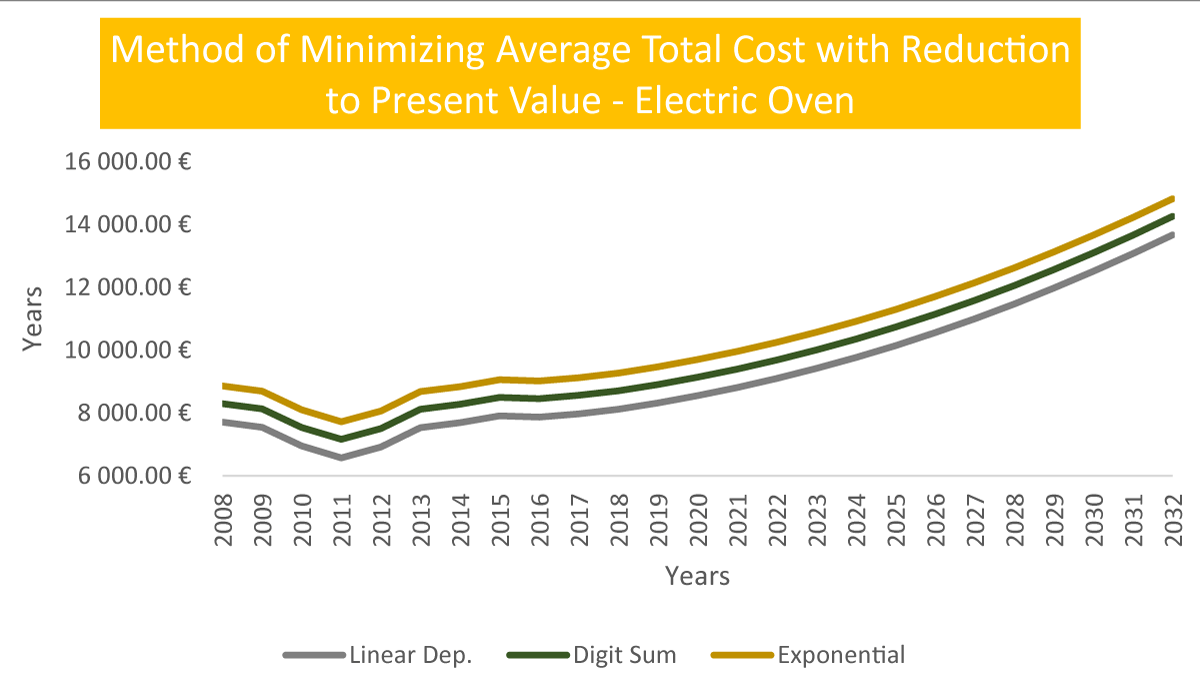
Figure 17: MCMT-RVP with variable apparent rate- Electric Oven.
| Table 14: MCMT - RVP with variable apparent rate – Electric Oven. | ||||
| Year | Method of Minimizing Average Total Cost- RVP | |||
| Civil | j | Linear Dep | Digit Sum | Exponential |
| 2008 | 0 | |||
| 2009 | 1 | 7 711,42 € | 8 298,24 € | 8 861,36 € |
| 2010 | 2 | 7 544,86 € | 8 131,68 € | 8 694,80 € |
| 2011 | 3 | 6 952,52 € | 7 539,33 € | 8 102,45 € |
| 2012 | 4 | 6 576,11 € | 7 162,93 € | 7 726,05 € |
| 2013 | 5 | 6 918,10 € | 7 504,92 € | 8 068,04 € |
| 2014 | 6 | 7 534,11 € | 8 120,92 € | 8 684,04 € |
| 2015 | 7 | 7 692,40 € | 8 279,22 € | 8 842,34 € |
| 2016 | 8 | 7 912,06 € | 8 498,88 € | 9 061,99 € |
| 2017 | 9 | 7 872,49 € | 8 459,30 € | 9 022,42 € |
| 2018 | 10 | 7 976,91 € | 8 563,73 € | 9 126,84 € |
| 2019 | 11 | 8 122,12 € | 8 708,94 € | 9 272,06 € |
| 2020 | 12 | 8 323,73 € | 8 910,55 € | 9 473,66 € |
| 2021 | 13 | 8 554,09 € | 9 140,91 € | 9 704,02 € |
| 2022 | 14 | 8 813,21 € | 9 400,03 € | 9 963,14 € |
| 2023 | 15 | 9 101,42 € | 9 688,24 € | 10 251,36 € |
| 2024 | 16 | 9 419,24 € | 10 006,06 € | 10 569,18 € |
| 2025 | 17 | 9 767,28 € | 10 354,10 € | 10 917,22 € |
| 2026 | 18 | 10 146,13 € | 10 732,94 € | 11 296,06 € |
| 2027 | 19 | 10 556,28 € | 11 143,10 € | 11 706,22 € |
| 2028 | 20 | 10 998,08 € | 11 584,90 € | 12 148,01 € |
| 2029 | 21 | 11 471,58 € | 12 058,40 € | 12 621,52 € |
| 2030 | 22 | 11 976,51 € | 12 563,33 € | 13 126,45 € |
| 2031 | 23 | 12 512,17 € | 13 098,99 € | 13 662,10 € |
| 2032 | 24 | 13 077,33 € | 13 664,14 € | 14 227,26 € |
| 2033 | 25 | 13 670,17 € | 14 256,99 € | 14 820,11 € |
Through the application of the defined methods and the results obtained, having considered an apparent constant rate, it is observed that the best time to replace the electric oven is the year 2019. This statement can be confirmed by the data previously mentioned; the same is no longer the case when using an apparent variable rate. In this case, the information available to us states that the best period to replace the electric oven is between 2012 and 2014. It is also important to note that the method used is different in both cases, because, when we refer to the year 2019, the method used was MCTM, for the years between 2012 and 2014 were MCMT - RVP and MRAU, respectively.
Ring oven
- Oven Characterization
On the nameplate, we can check the entire identity of the ring oven (Figure 18 a,b).
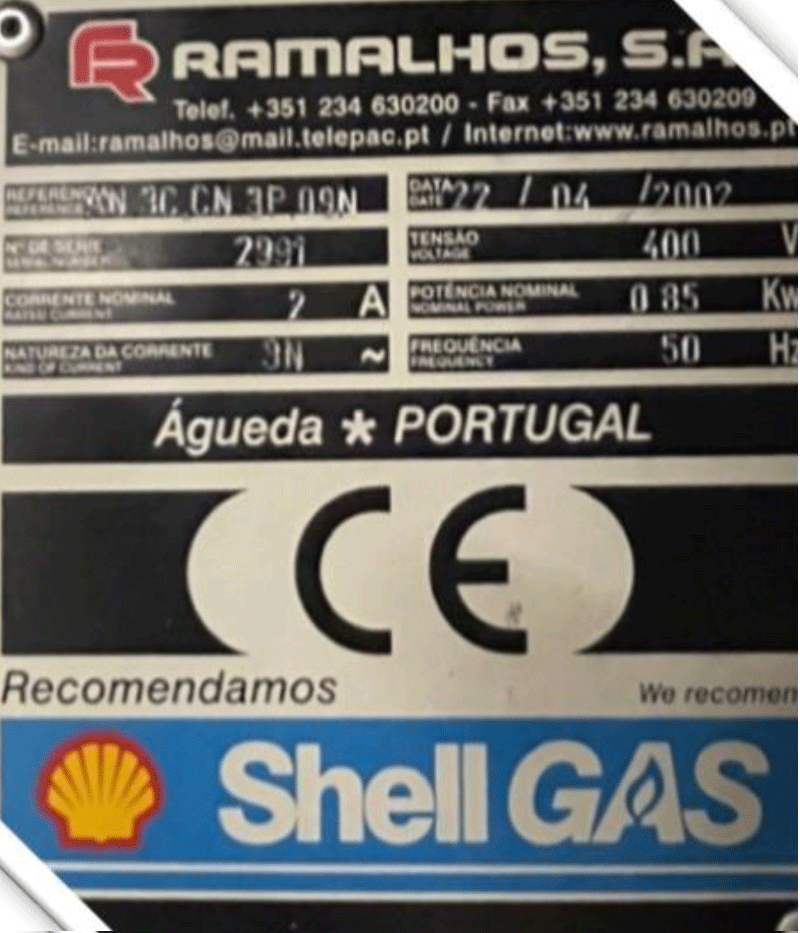
Figure 18a: Ring Oven characterization.
As can be seen, the furnace was installed in 2002, one of the first furnaces installed in the production area, being a piece of equipment approximately 20 years old. The nameplate does not show information on gas consumption. However, through the supplier’s catalogs, it was possible to choose a similar oven. Figures 18,19 illustrate the values relating to propane consumption.
The data from Table 15 was collected for the ring oven, and used for calculating asset replacement methods.
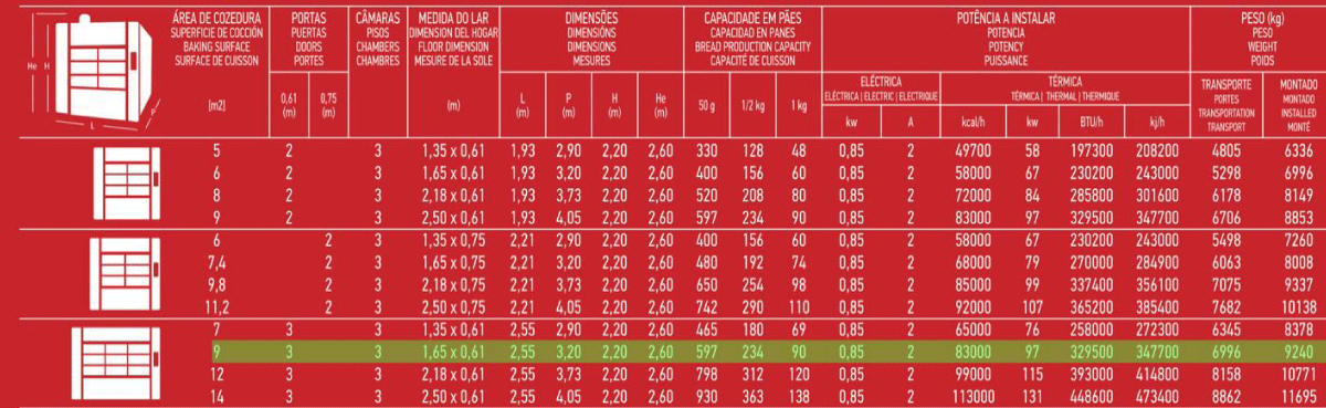
Figure 18b: Ring Oven characterization.
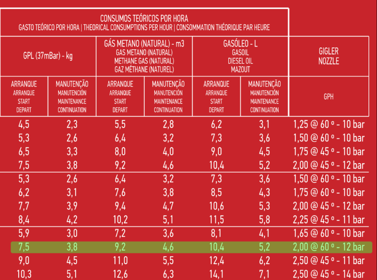
Figure 19: Ring Oven characterization.
| Table 15: Equipment History (Ring Oven). | |
Acquisition Cost: |
13.023,60 € |
Year of Installation: |
2002 |
Supplier/Manufacturer: |
Ramalhos |
Year (End of life): |
20 years |
Residual Value: |
500,00 € |
- Calculation of maintenance and operating costs
Again, at this point, due to the uncertainty of collected data regarding maintenance costs (Table 16), the following was considered:
| Table 16: Maintenance costs of the ring oven. | ||
| Ring Oven 3C/3P | ||
| Year | Type of Service | Cost |
| 2004 | Miscellaneous Equipment Repairs | 35,00 € |
| 2010 | Miscellaneous Equipment Repairs | 269,76 € |
| 2014 | Tempered Glass | 218,94 € |
| 2017 | Miscellaneous Equipment Repairs | 501,72 € |
| 2018 | Tempered Glass | 249,08 € |
| Factory Utensil Tools | 154,98 € | |
| Freight Transport | 12,30 € | |
- Since we have no real data concerning the cost of maintenance, it was assumed that, in the first year (2003), the maintenance cost was 1.500,00€ and, in 2004 and forward, had an increase of 10% compared to the average costs considered (based on historical data collected);
- The assumption of the average monthly cost of the electrical part (including hours of maintenance by the electrician, plus equipment) is shown in Table 17.
| Table 17: Average maintenance costs. | |
| Maintenance Costs | |
| Maintenance Costs - electrician | 600 |
| Average Cost (over the years – Historical) | 205,97 € |
| Total | 805,97 € |
In the ring oven was, again, only considered the energy costs; so, it was necessary to collect data on the variation of propane gas price over the years, through the database, a database of contemporary Portugal that provides this type of information.
It was considered that both worked 11 hours daily and only 361 days a year, as the company is closed all day on 25 and 26 December and 1 and 2 January (Table 18).
| Table 18: Gas Over operating costs. | ||
| Cost of operation | ||
| Number of hours worked | Start-up (hours) | 0,75 |
| Maintenance (hours) | 10,25 | |
| Total | 11 h | |
| Oven power | 49 kW/h | |
| Gas consumption | Starting | 7,5 kg |
Through the analysis of Table 18, we can forecast the estimated values of the cost of natural gas for the coming years. From the analysis of Table 19, one may notice that the oscillation of the operating costs is due to changes in the propane price from 2010 until now.
| Table 19: Maintenance Costs and Operation Costs of the Ring Oven. | |||||||||
| Years | Cost Electricity €/kw |
€*P | Operating Costs Electricity | €/kg Gas |
Operating Costs Gas | Operating Costs Total | Maintenance Cost | Total Costs | |
| 2002 | 0 | 0,1482 € | 0,1260 € | 45,48 € | 1,01 € | 16 252,49 € | 16 297,97 € | 16 297,97 € | |
| 2003 | 1 | 0,1508 € | 0,1282 € | 46,27 € | 1,12 € | 18 022,56 € | 18 068,84 € | 1 500,00 € | 19 568,84 € |
| 2004 | 2 | 0,1584 € | 0,1346 € | 48,61 € | 1,20 € | 19 309,89 € | 19 358,50 € | 873,98 € | 20 245,06 € |
| 2005 | 3 | 0,1654 € | 0,1406 € | 50,75 € | 1,34 € | 21 562,71 € | 21 613,46 € | 973,96 € | 22 588,69 € |
| 2006 | 4 | 0,1993 € | 0,1694 € | 61,16 € | 1,58 € | 25 424,69 € | 25 485,84 € | 1 071,36 € | 26 558,59 € |
| 2007 | 5 | 0,2081 € | 0,1769 € | 63,86 € | 1,66 € | 26 712,01 € | 26 775,87 € | 1 178,50 € | 27 955,89 € |
| 2008 | 6 | 0,2175 € | 0,1849 € | 66,74 € | 1,87 € | 30 091,25 € | 30 157,99 € | 1 296,35 € | 31 456,01 € |
| 2009 | 7 | 0,2279 € | 0,1937 € | 69,93 € | 1,67 € | 26 872,93 € | 26 942,86 € | 1 425,98 € | 28 370,68 € |
| 2010 | 8 | 0,2350 € | 0,1998 € | 72,11 € | 1,89 € | 30 413,08 € | 30 485,19 € | 1 568,58 € | 32 055,79 € |
| 2011 | 9 | 0,2284 € | 0,1941 € | 70,08 € | 2,08 € | 33 470,48 € | 33 540,56 € | 1 725,44 € | 35 268,23 € |
| 2012 | 10 | 0,2246 € | 0,1909 € | 68,92 € | 2,14 € | 34 435,97 € | 34 504,89 € | 1 897,98 € | 36 405,32 € |
| 2013 | 11 | 0,2453 € | 0,2085 € | 75,27 € | 2,05 € | 32 987,73 € | 33 063,00 € | 2 087,78 € | 35 153,47 € |
| 2014 | 12 | 0,2550 € | 0,2168 € | 78,25 € | 1,97 € | 31 700,40 € | 31 778,65 € | 2 296,55 € | 34 078,17 € |
| 2015 | 13 | 0,2647 € | 0,2250 € | 81,22 € | 1,90 € | 30 573,99 € | 30 655,22 € | 2 526,21 € | 33 184,69 € |
| 2016 | 14 | 0,2744 € | 0,2332 € | 84,20 € | 1,88 € | 30 252,16 € | 30 336,36 € | 2 778,83 € | 33 118,78 € |
| 2017 | 15 | 0,2841 € | 0,2415 € | 87,18 € | 2,03 € | 32 665,90 € | 32 753,07 € | 3 056,71 € | 35 813,74 € |
| 2018 | 16 | 0,2938 € | 0,2497 € | 90,15 € | 2,21 € | 35 562,38 € | 35 652,53 € | 3 362,39 € | 39 019,26 € |
| 2019 | 17 | 0,3035 € | 0,2580 € | 93,13 € | 2,26 € | 36 383,05 € | 36 476,18 € | 3 698,62 € | 40 179,58 € |
| 2020 | 18 | 0,3132 € | 0,2662 € | 96,11 € | 2,33 € | 37 429,00 € | 37 525,11 € | 4 068,49 € | 41 598,85 € |
| 2021 | 19 | 0,3229 € | 0,2745 € | 99,08 € | 2,39 € | 38 474,96 € | 38 574,04 € | 4 475,33 € | 43 055,16 € |
| 2022 | 20 | 0,3326 € | 0,2827 € | 102,06 € | 2,46 € | 39 520,91 € | 39 622,97 € | 4 922,87 € | 44 552,20 € |
Table 20 and Figure 20 shows the values for the three methods, namely, the Linear Depreciation Method, the Method Sum of Digits, and the Exponential Method.
| Table 20: Depreciation methods – Ring Oven. | ||||
| Year | Methods | |||
| j | Linear Dep. | Digit Sum | Exponential | |
| 2002 | 0 | 13 023,60 € | 13 023,60 € | 13 023,60 € |
| 2003 | 1 | 12 397,42 € | 11 830,88 € | 11 064,79 € |
| 2004 | 2 | 11 771,24 € | 10 697,79 € | 9 400,59 € |
| 2005 | 3 | 11 145,06 € | 9 624,34 € | 7 986,69 € |
| 2006 | 4 | 10 518,88 € | 8 610,52 € | 6 785,45 € |
| 2007 | 5 | 9 892,70 € | 7 656,34 € | 5 764,89 € |
| 2008 | 6 | 9 266,52 € | 6 761,80 € | 4 897,82 € |
| 2009 | 7 | 8 640,34 € | 5 926,89 € | 4 161,16 € |
| 2010 | 8 | 8 014,16 € | 5 151,62 € | 3 535,30 € |
| 2011 | 9 | 7 387,98 € | 4 435,99 € | 3 003,58 € |
| 2012 | 10 | 6 761,80 € | 3 779,99 € | 2 551,82 € |
| 2013 | 11 | 6 135,62 € | 3 183,63 € | 2 168,02 € |
| 2014 | 12 | 5 509,44 € | 2 646,90 € | 1 841,94 € |
| 2015 | 13 | 4 883,26 € | 2 169,81 € | 1 564,90 € |
| 2016 | 14 | 4 257,08 € | 1 752,36 € | 1 329,53 € |
| 2017 | 15 | 3 630,90 € | 1 394,54 € | 1 129,56 € |
| 2018 | 16 | 3 004,72 € | 1 096,36 € | 959,67 € |
| 2019 | 17 | 2 378,54 € | 857,82 € | 815,33 € |
| 2020 | 18 | 1 752,36 € | 678,91 € | 692,70 € |
| 2021 | 19 | 1 126,18 € | 559,64 € | 588,52 € |
| 2022 | 20 | 500,00 € | 500,00 € | 500,00 € |
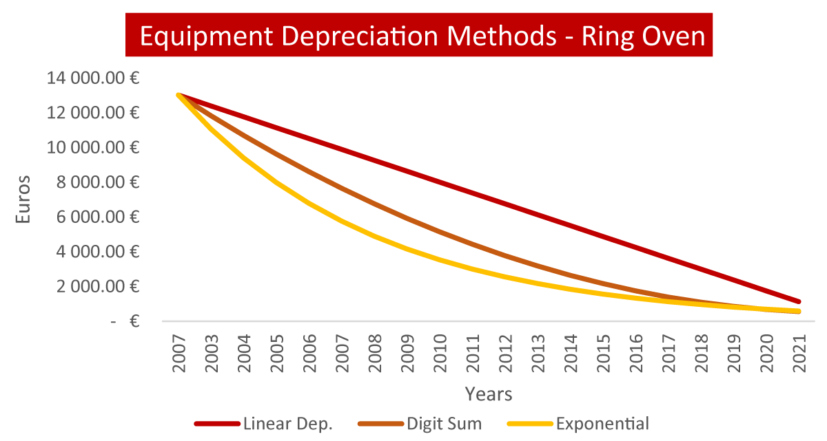
Figure 20: Depreciation methods – Ring Oven.
The study timeline for the equipment ring oven was 20 years, since, according to our experience, it is the maximum useful life of the equipment. Therefore, the timeline of this study will be from the moment of acquisition until the end of the equipment’s useful life, specifically, from 2002 (the year of acquisition) until 2022.
The annual depreciation quota of 626,18€ was obtained using the Linear Depreciation method. Under the Exponential method, the depreciation rate obtained was 15%.
Through the analysis of Table 20, it is possible to conclude that the Linear Depreciation method presents a slower decrease over time; the same is no longer seen in the others. It should be noted that, if we compare the method of the digital sum with the exponential method, the latter presents a much faster decay. These previously mentioned facts may also be seen in Figure 20.
With the aforementioned study, it was possible to process data related to the economic cycle of replacing the ring oven, which can be seen in Figure 20.
Constant apparent rate replacement methods – Ring Oven
- Uniform annual expenditure method (MRAU) – Ring Oven
Table 21 and Figure 21 show the results obtained by applying the method of uniform annual expenditure, and, through the analysis of Figure 22, it can be observed that both depreciation methods follow the same path and are very similar, tending to 2022 (33.326,45 €). However, it is noticed that the decision maker is unable to define an exact moment for the furnace replacement since no moment is identified where the annual outlay is minimal. It is important to mention, again, that the apparent rate is constant over the years, which may influence the final results.
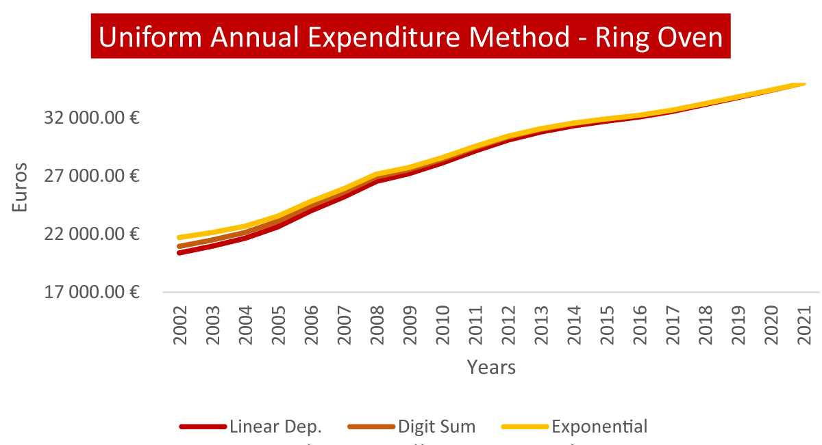
Figure 21: MRAU with variable apparent rate – Ring Oven.
Table 21: MRAU with constant apparent rate – Ring Oven. |
||||
| Years | Uniform Annual Expenditure Method | |||
| j | Linear Dep. | Digit Sum | Exponential | |
| 2002 | 0 | |||
| 2003 | 1 | 20 201,28 € | 20 773,49 € | 21 547,24 € |
| 2004 | 2 | 20 540,85 € | 21 085,64 € | 21 743,99 € |
| 2005 | 3 | 21 429,60 € | 21 946,68 € | 22 503,51 € |
| 2006 | 4 | 22 903,16 € | 23 392,24 € | 23 859,97 € |
| 2007 | 5 | 23 982,59 € | 24 443,37 € | 24 833,08 € |
| 2008 | 6 | 25 305,43 € | 25 737,61 € | 26 059,24 € |
| 2009 | 7 | 25 823,43 € | 26 226,72 € | 26 489,16 € |
| 2010 | 8 | 26 657,45 € | 27 031,55 € | 27 242,79 € |
| 2011 | 9 | 27 649,67 € | 27 994,28 € | 28 161,50 € |
| 2012 | 10 | 28 552,66 € | 28 867,49 € | 28 997,16 € |
| 2013 | 11 | 29 183,73 € | 29 468,46 € | 29 566,42 € |
| 2014 | 12 | 29 625,28 € | 29 879,62 € | 29 951,14 € |
| 2015 | 13 | 29 934,64 € | 30 158,27 € | 30 208,13 € |
| 2016 | 14 | 30 195,82 € | 30 388,44 € | 30 420,95 € |
| 2017 | 15 | 30 589,99 € | 30 751,28 € | 30 770,40 € |
| 2018 | 16 | 31 120,97 € | 31 250,63 € | 31 259,92 € |
| 2019 | 17 | 31 652,71 € | 31 750,42 € | 31 753,15 € |
| 2020 | 18 | 32 197,97 € | 32 263,43 € | 32 262,59 € |
| 2021 | 19 | 32 756,02 € | 32 788,91 € | 32 787,24 € |
| 2022 | 20 | 33 326,45 € | 33 326,45 € | 33 326,45 € |
- Method of minimizing average total cost (MCMT) – Ring Oven
By analyzing Table 22 and Figure 22, and through the values obtained by the studied methods for Minimizing Average Total Cost, it can be concluded that the year of replacement is 2005 since the three methods have minimum values in that same year. In this case, through the values obtained, the decision maker would have greater certainty about the best time to replace the equipment.
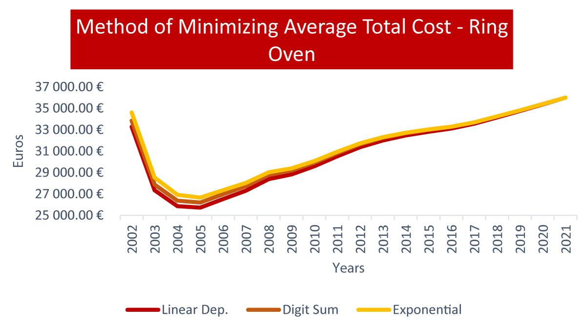
Figure 22: MCMT with constant apparent rate – Ring Oven.
| Table 22: MCMT with constant apparent rate – Ring Oven. | ||||
| Year | Method of Minimizing Average Total Cost | |||
| j | Linear Dep. | Digit Sum | Exponential | |
| 2002 | 0 | |||
| 2003 | 1 | 33 218,62 € | 33 785,16 € | 34 551,25 € |
| 2004 | 2 | 27 044,93 € | 27 581,65 € | 28 230,26 € |
| 2005 | 3 | 25 768,24 € | 26 275,15 € | 26 821,03 € |
| 2006 | 4 | 26 122,37 € | 26 599,46 € | 27 055,73 € |
| 2007 | 5 | 26 614,31 € | 27 061,58 € | 27 439,87 € |
| 2008 | 6 | 27 525,62 € | 27 943,08 € | 28 253,74 € |
| 2009 | 7 | 27 735,80 € | 28 123,44 € | 28 375,68 € |
| 2010 | 8 | 28 354,07 € | 28 711,89 € | 28 913,93 € |
| 2011 | 9 | 29 191,89 € | 29 519,89 € | 29 679,04 € |
| 2012 | 10 | 29 975,85 € | 30 274,03 € | 30 396,85 € |
| 2013 | 11 | 30 503,47 € | 30 771,83 € | 30 864,16 € |
| 2014 | 12 | 30 853,54 € | 31 092,09 € | 31 159,17 € |
| 2015 | 13 | 31 081,03 € | 31 289,75 € | 31 336,29 € |
| 2016 | 14 | 31 271,31 € | 31 450,22 € | 31 480,42 € |
| 2017 | 15 | 31 615,88 € | 31 764,97 € | 31 782,64 € |
| 2018 | 16 | 32 117,73 € | 32 237,00 € | 32 245,55 € |
| 2019 | 17 | 32 628,79 € | 32 718,25 € | 32 720,74 € |
| 2020 | 18 | 33 161,92 € | 33 221,55 € | 33 220,79 € |
| 2021 | 19 | 33 715,57 € | 33 745,39 € | 33 743,87 € |
| 2022 | 20 | 34 288,71 € | 34 288,71 € | 34 288,71 € |
- Method of Minimizing Average Total Cost with Reduction to Present Value (MCMT-RVP) – Electric Oven
Through the analysis of Table 23 and Figure 23, it is possible to observe that the lowest average cost of the equipment is not reached, as the period in which it occurs is not visible. It is difficult for the decision maker to make a decision regarding the replacement of the equipment based on this method since there is no objective moment that indicates the lowest average cost of the equipment.
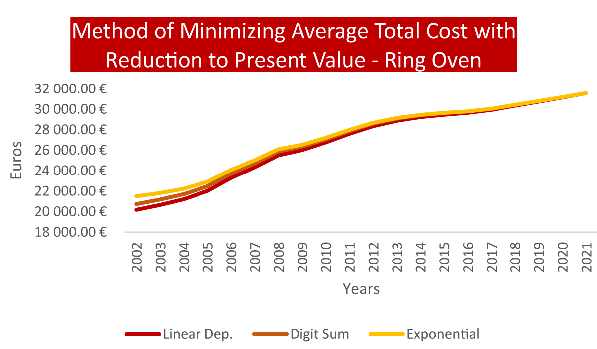
Figure 23: MCMT - RVP with constant apparent rate – Ring Oven.
| Table 23: MCMT - RVP with constant apparent rate – Ring Oven. | ||||
| Year | Method of Minimizing Average Total Cost - RVP | |||
| j | Linear Dep. | Digit Sum | Exponential | |
| 2002 | 0 | |||
| 2003 | 1 | 20 124,01 € | 20 684,95 € | 21 443,45 € |
| 2004 | 2 | 20 352,77 € | 20 878,92 € | 21 514,74 € |
| 2005 | 3 | 21 117,30 € | 21 609,30 € | 22 139,13 € |
| 2006 | 4 | 22 395,76 € | 22 854,23 € | 23 292,70 € |
| 2007 | 5 | 23 375,60 € | 23 801,16 € | 24 161,09 € |
| 2008 | 6 | 24 532,34 € | 24 925,60 € | 25 218,26 € |
| 2009 | 7 | 24 903,77 € | 25 265,32 € | 25 500,60 € |
| 2010 | 8 | 25 573,43 € | 25 903,87 € | 26 090,45 € |
| 2011 | 9 | 26 386,71 € | 26 686,61 € | 26 832,13 € |
| 2012 | 10 | 27 107,14 € | 27 377,08 € | 27 488,26 € |
| 2013 | 11 | 27 563,83 € | 27 804,37 € | 27 887,13 € |
| 2014 | 12 | 27 837,91 € | 28 049,61 € | 28 109,14 € |
| 2015 | 13 | 27 985,52 € | 28 168,92 € | 28 209,80 € |
| 2016 | 14 | 28 086,50 € | 28 242,15 € | 28 268,42 € |
| 2017 | 15 | 28 309,02 € | 28 437,43 € | 28 452,65 € |
| 2018 | 16 | 28 654,79 € | 28 756,51 € | 28 763,80 € |
| 2019 | 17 | 28 997,50 € | 29 073,03 € | 29 075,14 € |
| 2020 | 18 | 29 348,79 € | 29 398,65 € | 29 398,01 € |
| 2021 | 19 | 29 707,87 € | 29 732,55 € | 29 731,29 € |
| 2022 | 20 | 30 074,22 € | 30 074,22 € | 30 074,22 € |
Variable apparent rate replacement methods – Ring Oven
- Uniform Annual Expenditure Method (MRAU) – Ring Oven
Table 24 and Figure 24 show the results obtained by applying the method of uniform annual expenditure. It is observed that, through the application of the method, there is a large deviation in the results in all methods used. When observing the figure below (Figure 24), it appears that the decision-maker can define a time for the replacement of the furnace in 2009, that is, it is where the minimum value, given by the annual expenditure method, occurs, which transmits to the decision maker the best time for replacing the furnace equipment.
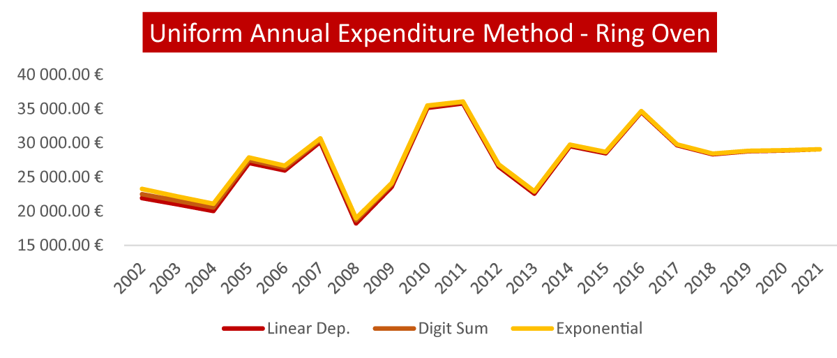
Figure 24: MRAU with constant apparent rate - Ring Oven.
| Table 24: MRAU with constant apparent rate - Ring Oven. | ||||
| Year | Uniform Annual Expenditure Method | |||
| j | Linear Dep. | Digit Sum | Exponential | |
| 2002 | 0 | |||
| 2003 | 1 | 21 869,85 € | 22 436,40 € | 23 202,49 € |
| 2004 | 2 | 20 704,11 € | 21 224,85 € | 21 854,13 € |
| 2005 | 3 | 19 959,71 € | 20 466,01 € | 21 011,23 € |
| 2006 | 4 | 27 390,90 € | 27 790,48 € | 28 172,63 € |
| 2007 | 5 | 26 042,92 € | 26 410,11 € | 26 720,67 € |
| 2008 | 6 | 30 319,62 € | 30 605,90 € | 30 818,94 € |
| 2009 | 7 | 17 354,45 € | 17 795,80 € | 18 082,99 € |
| 2010 | 8 | 22 733,60 € | 23 090,92 € | 23 292,68 € |
| 2011 | 9 | 34 030,28 € | 34 254,82 € | 34 363,77 € |
| 2012 | 10 | 34 628,50 € | 34 820,13 € | 34 899,06 € |
| 2013 | 11 | 25 440,40 € | 25 677,11 € | 25 758,55 € |
| 2014 | 12 | 21 407,76 € | 21 664,26 € | 21 736,39 € |
| 2015 | 13 | 27 844,29 € | 28 024,62 € | 28 064,82 € |
| 2016 | 14 | 26 776,66 € | 26 938,23 € | 26 965,51 € |
| 2017 | 15 | 32 521,07 € | 32 630,70 € | 32 643,69 € |
| 2018 | 16 | 28 034,24 € | 28 137,50 € | 28 144,90 € |
| 2019 | 17 | 26 768,69 € | 26 851,54 € | 26 853,86 € |
| 2020 | 18 | 27 173,53 € | 27 229,36 € | 27 228,64 € |
| 2021 | 19 | 27 270,36 € | 27 298,96 € | 27 297,50 € |
| 2022 | 20 | 27 411,80 € | 27 411,80 € | 27 411,80 € |
- Method of Minimizing Average Total Cost with Reduction to Present Value (MCMT-RVP) – Electric Oven
Table 25 and Figure 25 shows that the lowest average cost of the equipment appears in 2008, being verifiable in all methods applied in the period under study. The results obtained facilitate the decision regarding the replacement of the equipment.
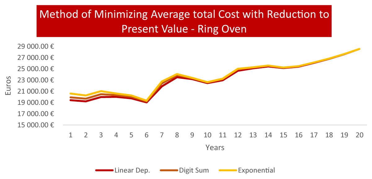
Figure 25: MCMT - RVP with variable apparent rate - Ring Oven.
| Table 25: MCMT - RVP with variable apparent rate - Ring Oven | ||||
| Year | Method of Minimizing Average Total Cost- RVP | |||
| j | Linear Dep. | Digit Sum | Exponential | |
| 2002 | 0 | |||
| 2003 | 1 | 19 377,86 € | 19 879,85 € | 20 558,64 € |
| 2004 | 2 | 18 942,21 € | 19 418,64 € | 19 994,37 € |
| 2005 | 3 | 19 911,90 € | 20 416,99 € | 20 960,91 € |
| 2006 | 4 | 20 263,12 € | 20 566,86 € | 20 857,34 € |
| 2007 | 5 | 19 805,31 € | 20 084,55 € | 20 320,73 € |
| 2008 | 6 | 19 134,32 € | 19 314,98 € | 19 449,43 € |
| 2009 | 7 | 20 824,63 € | 21 354,23 € | 21 698,85 € |
| 2010 | 8 | 22 692,74 € | 23 049,41 € | 23 250,81 € |
| 2011 | 9 | 22 458,45 € | 22 606,64 € | 22 678,54 € |
| 2012 | 10 | 21 742,54 € | 21 862,86 € | 21 912,42 € |
| 2013 | 11 | 22 028,83 € | 22 233,81 € | 22 304,32 € |
| 2014 | 12 | 23 379,31 € | 23 659,43 € | 23 738,20 € |
| 2015 | 13 | 23 678,00 € | 23 831,35 € | 23 865,54 € |
| 2016 | 14 | 23 905,14 € | 24 049,39 € | 24 073,74 € |
| 2017 | 15 | 23 689,48 € | 23 769,34 € | 23 778,80 € |
| 2018 | 16 | 23 998,66 € | 24 087,05 € | 24 093,39 € |
| 2019 | 17 | 24 611,39 € | 24 687,56 € | 24 689,69 € |
| 2020 | 18 | 25 284,99 € | 25 336,94 € | 25 336,27 € |
| 2021 | 19 | 26 057,36 € | 26 084,69 € | 26 083,30 € |
| 2022 | 20 | 26 936,33 € | 26 936,33 € | 26 936,33 € |
Final conclusion: Through the application of the methods presented in this project and the results obtained (constant apparent rate), it is observed that the best time to replace the annular furnace is the year 2006. The same does not happen when we use a variable apparent rate, as it refers to the replacement of the equipment between the years 2008 and 2009. The method used is different in both cases, because when we refer to the year 2006, the method used was the MCTM and, for the years 2008 and 2009 the MRAU and the MCMT - RVP, respectively. The methods used above have been used in other cases such as the one presented by De Almeida Pais, et al. [10], Farinha [20], Farinha, et al. [16], Raposo, et al. [21], Raposo, et al. [24], Raposo, et al. [22] and Raposo, et al. [23], which present several case studies, namely in hospital equipment, water abstractions (water sector) and in a fleet of urban buses (transport sector).
This paper presents an approach to energy efficiency and to the econometric models, whether by the analysis of an asset’s life cycle in determining the most rational time for its replacement in the food industry. The economic aspects were guided by relevant cash flow indicators using, for this, the costs associated with the acquisition, operation, and maintenance, among others.
The approach presented in this paper allows, from the outset, monitor the equipment’s life cycle by the managers and is clearly a powerful decision-support tool for this sector.
The study started with the collection and analysis of data, namely, energy costs (electricity and gas), costs of maintenance, and production of the organization’s physical assets. We found that the absence of asset management software in the company, where the case study was carried out, made it difficult to collect and analyze the historical data of the various equipment; so, it was necessary to extrapolate some data.
Therefore, it can be concluded that the company must invest and acquire software, as well as monitoring equipment, which allows obtaining more reliable data regarding costs (maintenance and production), energy consumption, and expenses and, consequently, to evolve the management of the company’s assets, allowing verification and analysis of the data to reduce costs, reduce energy consumption and expenses.
Being the present study focused on econometric models for determining the more rational moment of a furnace replacement in food companies, the outcome resulted in a model for decision support by following the LCC of food cooking ovens, aimed at the definition of the most appropriate time to replace them; however, it has the potential to extend to other types of equipment.
The conducting threads of the research carried out aimed at rationalizing the management of the life cycle of physical assets and the time for the replacement of equipment / ovens.
In this context, it was found that, through the econometric models studied, the most appropriate moment can be obtained for the replacement of bakery ovens. It is important to mention that these ovens have very different characteristics, since each one has its own energy source: in the electric oven, through the MCMT, with a constant apparent rate, it was observed that the best time would be the year 2019; however, when the apparent rate is variable, the same is no longer the case, as it refers to an interval of years, that is, between 2012 and 2014, using the MCMT-RVT and MRAU methods, respectively. In the case of the ring oven (gas), it was observed that, by the MCMT method, with constant apparent rate, the most appropriate moment for its replacement corresponds to the year 2006; with variable apparent rate, points to the range of values between the years 2008 and 2009, using the MCMT-RVP and MRAU methods, respectively.
Regarding the study carried out on the energy efficiency of the assets, it was possible to verify that there is a big fluctuation in consumption, which concerns the main sources of energy used. It is important to note that the energy source with the highest consumption is propane gas since it is where the highest consumption occurs. It was also possible to identify that the highest consumption of electricity occurs in the summer months, due to the higher average ambient temperature and the refrigerated areas requiring greater energy consumption to maintain the internal temperature. It was also observed that the consumption of the main sources of energy increased until 2018. However, due to some alerts and measures implemented, it was possible to reduce their consumption in 2019, with the expectation that in 2020 it will be even lower. It is necessary, for the company, to create new models/documents that allow rigorous analysis of its assets, including energy consumption, in order to make the company more energy efficient.
The present study demonstrates that the monitoring and analysis of the life cycle of physical assets can bring enormous advantages to the managers of this type of industry, allowing, by this way, more efficient management of the equipment, increasing its availability and efficiency, and contributing to an increase on the productivity of companies and the quality of their products.
Author contributions
Conceptualization, J.P., J.T.F. and H.R.; methodology, J.P., J.T.F. and H.R.; formal analysis, J.T.F., and H.R.; investigation, J.P.; resources, T.F. and H.R.; writing—original draft preparation, J.P.; writing—review and editing, J.T.F., H.R. and E.P.; project administration, J.T.F., and H.R.; funding acquisition, J.T.F., and H.R. All authors have read and agreed to the published version of the manuscript.
Funding
Please add: “This research received no external funding” “This research was funded by NAME OF FUNDER, grant number XXX” and “The APC was funded by XXX”. Check carefully that the details given are accurate and use the standard spelling of funding agency names at https://search.crossref.org/funding. Any errors may affect your future funding.
- Pais E, Farinha T, Raposo H. ISO55001 – A Pragmatic Proposal for Diagnosis and Implementation. Proceedings IRF2020: 7th International Conference Integrity-Reliability-Failure. JF. Silva Gomes and SA. Meguid (editors), INEGI-FEUP. 2020; 739-742. https://paginas.fe.up.pt/~irf/Proceedings_IRF2020/
- Siksnelyte I, Zavadskas EK, Streimikiene D, Sharma D. An Overview of Multi-Criteria Decision-Making Methods in Dealing with Sustainable Energy Development Issues. Energies. 2018; 11:2754. http://dx.doi.org/10.3390/en11102754.
- Taghizadeh-Hesary F, Yoshino N. Sustainable Solutions for Green Financing and Investment in Renewable Energy Projects. Energies. 2020; 13(1): 788. https://doi.org/10.3390/en13040788.
- Yumashev A, Slusarczyk B, Kondrashev S, Mikhaylov A. Global Indicators of Sustainable Development: Evaluation of the Influence of the Human Development Index on Consumption and Quality of Energy. Energies. 2020; 13(1): 2768. https://doi.org/10.3390/en13112768.
- Martins AB, Farinha JT, Cardoso AM. Calibration and Certification of Industrial Sensors—A Global Review. WSEAS Trans. Syst. Control. 2020; 15: 394–416. http://dx.doi.org/10.37394/23203.2020.15.41.
- Pais E, Farinha JT, Cardoso AJM, Raposo H. Optimizing the Life Cycle of Physical Assets. WSEAS Transactions on Systems and Control. 2020; 15(1): 417-430. http://dx.doi.org/10.37394/23203.2020.15.42.
- Balduíno M, Farinha JT, Cardoso AM. Production Optimization versus Asset Availability—A Review. WSEAS Trans. Syst. Control. 2020; 15 (1): 320–332. http://dx.doi.org/10.37394/23203.2020.15.33.
- Rodrigues J, Farinha JT, Cardoso AM. Predictive Maintenance Tools—A Global Survey. WSEAS Trans Syst Control. 2021; 16 (1): 96–109. http://dx.doi.org/10.37394/23203.2021.16.7.
- Rodrigues J, Costa I, Torres Farinha J, Mendes M, Margalho L. Predicting motor oil condition using artificial neural networks and principal component analysis. Maintenance and Reliability. 2020; 22 (3): 440–448. http://dx.doi. org/10.17531/ein.2020.3.6.
- de Almeida Pais JE, Raposo HDN, Farinha JT, Cardoso AJM, Marques PA. Optimizing the Life Cycle of Physical Assets through an Integrated Life Cycle Assessment Method. Energies. 2021; 14(1): 6128. https://doi.org/10.3390/en14196128.
- ISO 50001:2018 2018. Energy management systems – Requirements with guidance for use. https://www.iso.org/obp/ui/#iso:std:iso:50001:ed-2:v1:en .
- Mamala J, Graba M, Bieniek A, Prażnowski K, Augustynowicz A, Śmieja M. 2021. Study of energy consumption of a hybrid vehicle in real-world conditions. Maintenance and Reliability. 2021; 23 (4): 636–645. http://doi.org/10.17531/ein.2021.4.6.
- Kosucki A, Stawiński Ł, Malenta P, Zaczyński J, Skowrońska J. 2020. Energy consumption and energy efficiency improvement of overhead crane’s mechanisms. Maintenance and Reliability. 2020; 22(2):323–330. http://dx.doi.org/10.17531/ein.2020.2.15.
- Energy Efficiency 2019. International Energy Agency. https://iea.blob.core.windows.net/assets/8441ab46-9d86-47eb-b1fc-cb36fc3e7143/Energy_Efficiency_2019.pdf.
- Aragón CS, Pamplona E, Medina JRV. Identification of Investments in Energy Efficiency and its risk assessment. Management and Production. São Carlos. 2013; 20 (3): 525 – 536.
- Farinha JT, Raposo H, Galar D. Life Cycle Cost versus Life Cycle Investment – A new approach. WSEAS Transactions on Systems and Control. 2020; 15 (1): 743-753. http://dx.doi.org/10.37394/23203.2020.15.75.
- ISO 55000:2024 2014. Asset management – Overview, principles and terminology; ISO55001:2014 – Asset management – Management systems – Requirements; ISO 55002:2014 – Asset management – Management systems – Guidelines for application of ISO 550001.
- Pais E, Raposo H, Meireles A, Farinha JT. ISO55001 – A Strategic Tool for the Circular Economy – Diagnosis of the Organization´s State. Journal of Industrial Engineering and Management 2018. 2019. 1 (1): 89 - 108.
- Oliveira AE. The replacement of capital goods: an optimization model from the perspective of Production Engineering. Management and Production. São Carlos. 2015; 22 (3): 525–538.
- Farinha JMT. Asset Maintenance Engineering Methodologies (1st ed.). CRC Press. 2018. https://doi.org/10.1201/9781315232867.
- Raposo H, Farinha JT, Ferreira L, Galar D. An Integrated econometric model for bus replacement and determination of reserve fleet size based on predictive maintenance. Maintenance and Reliability. 2017; 19(3): 358-368. http://dx.doi.org/10.17531/ein.2017.3.6.
- Raposo H, Farinha JT, Pais E, Galar D. An Integrated Model for Dimensioning the Reserve Fleet based on the Maintenance Policy. WSEAS Transactions on Systems and Control. 2021; 16 (1): 43 – 65.
- Raposo H, Farinha T, Fonseca I, Galar D. Economic Life Cycle versus Lifespan – A Case Study of an Urban Bus Fleet. Engineering and Applied Sciences. 2019. http://dx.doi.org/10.11648/j.eas.20190402.12.
- Raposo H, Farinha JT, Ferreira L, Didelet F. Economic life cycle of the bus fleet: a case study. International Journal of Heavy Vehicle Systems. 2019; 26 (1): 31. DOI: 10.1504/IJHVS.2019.10018194.